From 1970 to 2020, the U.S. population increased by 63 percent, and the size of the U.S. economy increased by more than 3.8-fold. Since the 1970s, however, the United States, using a variety of anti-pollution policies, has made genuine progress against a number of pollutants. Table 12.1 lists the change in carbon dioxide emissions by energy users (from residential to industrial) according to the U.S. Energy Information Administration (EIA). The table shows that emissions of certain key air pollutants declined substantially from 2007 to 2012. They dropped 740 million metric tons (MMT) a year—a 12% reduction. This seems to indicate that there has been progress made in the United States in reducing overall carbon dioxide emissions, which contribute to the greenhouse effect.

Table 12.1 Carbon Dioxide Emissions from Energy Consumption, by Source (Source: EIA Monthly Energy Review)

Despite the gradual reduction in emissions from fossil fuels, many important environmental issues remain. Along with the still high levels of air and water pollution, other issues include hazardous waste disposal, destruction of wetlands and other wildlife habitats, and the impact on human health from pollution.

Externalities

Private markets, such as the cell phone industry, offer an efficient way to put buyers and sellers together and determine what goods they produce, how they produce them and who gets them. The principle that voluntary exchange benefits both buyers and sellers is a fundamental building block of the economic way of thinking. However, what happens when a voluntary exchange affects a third party who is neither the buyer nor the seller?

As an example, consider a concert producer who wants to build an outdoor arena that will host country music concerts a half-mile from your neighborhood. You will be able to hear these outdoor concerts while sitting on your back porch—or perhaps even in your dining room. In this case, the sellers and buyers of concert tickets may both be quite satisfied with their voluntary exchange, but you have no voice in their market transaction. The effect of a market exchange on a third party who is outside or “external” to the exchange is called an externality. Because externalities that occur in market transactions affect other parties beyond those involved, they are sometimes called spillovers.

Externalities can be negative or positive. If you hate country music, then having it waft into your house every night would be a negative externality. If you love country music, then what amounts to a series of free concerts would be a positive externality.

Pollution as a Negative Externality

Pollution is a negative externality. Economists illustrate the social costs of production with a demand and supply diagram. The social costs include the private costs of production that a company incurs and the external costs of pollution that pass on to society. Figure 12.2 shows the demand and supply for manufacturing refrigerators. The demand curve (D) shows the quantity demanded at each price. The supply curve (S_private) shows the quantity of refrigerators that all firms in the industry supply at each price assuming they are taking only their private costs into account and they are allowed to emit pollution at zero cost. The market equilibrium (E₀), where quantity supplied equals quantity demanded, is at a price of $650 per refrigerator and a quantity of 45,000 refrigerators. Table 12.2 reflects this information in the first three columns.

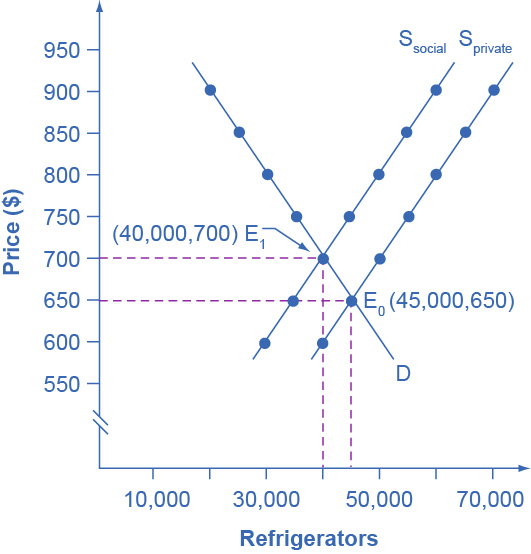
Figure 12.2 Taking Social Costs into Account: A Supply Shift If the firm takes only its own costs of production into account, then its supply curve will be S_private, and the market equilibrium will occur at E₀. Accounting for additional external costs of $100 for every unit produced, the firm’s supply curve will be S_social. The new equilibrium will occur at E₁.

Table 12.2 A Supply Shift Caused by Pollution Costs

However, as a by-product of the metals, plastics, chemicals and energy that refrigerator manufacturers use, some pollution is created. Let’s say that, if these pollutants were emitted into the air and water, they would create costs of $100 per refrigerator produced. These costs might occur because of adverse effects on human health, property values, or wildlife habitat, reduction of recreation possibilities, or because of other negative impacts. In a market with no anti-pollution restrictions, firms can dispose of certain wastes absolutely free. Now imagine that firms which produce refrigerators must factor in these external costs of pollution—that is, the firms have to consider not only labor and material costs, but also the broader costs to society of harm to health and other costs caused by pollution. If the firm is required to pay $100 for the additional external costs of pollution each time it produces a refrigerator, production becomes more costly and the entire supply curve shifts up by $100.

As Table 12.2 and Figure 12.2 illustrate, the firm will need to receive a price of $700 per refrigerator and produce a quantity of 40,000—and the firm’s new supply curve will be S_social. The new equilibrium will occur at E₁. In short, taking the additional external costs of pollution into account results in a higher price, a lower quantity of production, and a lower quantity of pollution. The following Work It Out feature will walk you through an example, this time with musical accompaniment.

Remember that the supply curve is based on choices about production that firms make while looking at their marginal costs, while the demand curve is based on the benefits that individuals perceive while maximizing utility. If no externalities existed, private costs would be the same as the costs to society as a whole, and private benefits would be the same as the benefits to society as a whole. Thus, if no externalities existed, the interaction of demand and supply will coordinate social costs and benefits.

However, when the externality of pollution exists, the supply curve no longer represents all social costs. Because externalities represent a case where markets no longer consider all social costs, but only some of them, economists commonly refer to externalities as an example of market failure. When there is market failure, the private market fails to achieve efficient output, because either firms do not account for all costs incurred in the production of output and/or consumers do not account for all benefits obtained (a positive externality). In the case of pollution, at the market output, social costs of production exceed social benefits to consumers, and the market produces too much of the product.

We can see a general lesson here. If firms were required to pay the social costs of pollution, they would create less pollution but produce less of the product and charge a higher price. In the next module, we will explore how governments require firms to account for the social costs of pollution.

Access for free at https://openstax.org/books/principles-economics-3e