67 The Building Blocks of Keynesian Analysis
Laura Prince and OpenStax
Learning Objectives
By the end of this section, you will be able to:
- Evaluate the Keynesian view of recessions through an understanding of sticky wages and prices and the importance of aggregate demand
- Explain the coordination argument, menu costs, and macroeconomic externality
- Analyze the impact of the expenditure multipler
Now that we have a clear understanding of what constitutes aggregate demand, we return to the Keynesian argument using the model of aggregate demand/aggregate supply (AD/AS). (For a similar treatment using Keynes’ income-expenditure model, see the appendix on The Expenditure-Output Model.)
Keynesian economics focuses on explaining why recessions and depressions occur and offering a policy prescription for minimizing their effects. The Keynesian view of recession is based on two key building blocks. First, aggregate demand is not always automatically high enough to provide firms with an incentive to hire enough workers to reach full employment. Second, the macroeconomy may adjust only slowly to shifts in aggregate demand because of sticky wages and prices, which are wages and prices that do not respond to decreases or increases in demand. We will consider these two claims in turn, and then see how they are represented in the AD/AS model.
The first building block of the Keynesian diagnosis is that recessions occur when the level of demand for goods and services is less than what is produced when labor is fully employed. In other words, the intersection of aggregate supply and aggregate demand occurs at a level of output less than the level of GDP consistent with full employment. Suppose the stock market crashes, as in 1929, or suppose the housing market collapses, as in 2008. In either case, household wealth will decline, and consumption expenditure will follow. Suppose businesses see that consumer spending is falling or face restrictions from a pandemic that curtail their operations. That will reduce expectations of the profitability of investment, so businesses will decrease investment expenditure.
This seemed to be the case during the Great Depression, since the physical capacity of the economy to supply goods did not alter much. No flood or earthquake or other natural disaster ruined factories in 1929 or 1930. No outbreak of disease decimated the ranks of workers. No key input price, like the price of oil, soared on world markets. The U.S. economy in 1933 had just about the same factories, workers, and state of technology as it had had four years earlier in 1929—and yet the economy had shrunk dramatically. This also seems to be what happened in 2008.
As Keynes recognized, the events of the Depression contradicted Say’s law that “supply creates its own demand.” Although production capacity existed, the markets were not able to sell their products. As a result, real GDP was less than potential GDP.
Link It Up
Visit this website for raw data used to calculate GDP.
Wage and Price Stickiness
Keynes also pointed out that although AD fluctuated, prices and wages did not immediately respond as economists often expected. Instead, prices and wages are “sticky,” making it difficult to restore the economy to full employment and potential GDP. Keynes emphasized one particular reason why wages were sticky: the coordination argument. This argument points out that, even if most people would be willing—at least hypothetically—to see a decline in their own wages in bad economic times as long as everyone else also experienced such a decline, a market-oriented economy has no obvious way to implement a plan of coordinated wage reductions. Unemployment proposed a number of reasons why wages might be sticky downward, most of which center on the argument that businesses avoid wage cuts because they may in one way or another depress morale and hurt the productivity of the existing workers.
Some modern economists have argued in a Keynesian spirit that, along with wages, other prices may be sticky, too. Many firms do not change their prices every day or even every month. When a firm considers changing prices, it must consider two sets of costs. First, changing prices uses company resources: managers must analyze the competition and market demand and decide the new prices, they must update sales materials, change billing records, and redo product and price labels. Second, frequent price changes may leave customers confused or angry—especially if they discover that a product now costs more than they expected. These costs of changing prices are called menu costs—like the costs of printing a new set of menus with different prices in a restaurant. Prices do respond to forces of supply and demand, but from a macroeconomic perspective, the process of changing all prices throughout the economy takes time.
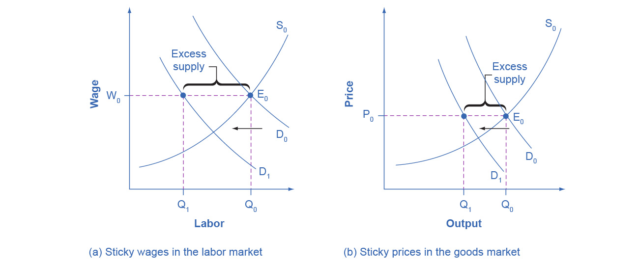
To understand the effect of sticky wages and prices in the economy, consider Figure 25.4 (a) illustrating the overall labor market, while Figure 25.4 (b) illustrates a market for a specific good or service. The original equilibrium (E0) in each market occurs at the intersection of the demand curve (D0) and supply curve (S0). When aggregate demand declines, the demand for labor shifts to the left (to D1) in Figure 25.4 (a) and the demand for goods shifts to the left (to D1) in Figure 25.4 (b). However, because of sticky wages and prices, the wage remains at its original level (W0) for a period of time and the price remains at its original level (P0).
As a result, a situation of excess supply—where the quantity supplied exceeds the quantity demanded at the existing wage or price—exists in markets for both labor and goods, and Q1 is less than Q0 in both Figure 25.4 (a) and Figure 25.4 (b). When many labor markets and many goods markets all across the economy find themselves in this position, the economy is in a recession; that is, firms cannot sell what they wish to produce at the existing market price and do not wish to hire all who are willing to work at the existing market wage. The Clear It Up feature discusses this problem in more detail.
Figure 25.4 Sticky Prices and Falling Demand in the Labor and Goods Market In both (a) and (b), demand shifts left from D0 to D1. However, the wage in (a) and the price in (b) do not immediately decline. In (a), the quantity demanded of labor at the original wage (W0) is Q0, but with the new demand curve for labor (D1), it will be Q1. Similarly, in (b), the quantity demanded of goods at the original price (P0) is Q0, but at the new demand curve (D1) it will be Q1. An excess supply of labor will exist, which we call unemployment. An excess supply of goods will also exist, where the quantity demanded is substantially less than the quantity supplied. Thus, sticky wages and sticky prices, combined with a drop in demand, bring about unemployment and recession.
Clear It Up
Why Was the Pace of Wage Adjustments Slow?
The recovery after the Great Recession in the United States was slow. In fact, many low-wage workers at McDonalds, Dominos, and Walmart threatened to strike for higher wages. Their plight was part of a larger trend in job growth and pay in the post–recession recovery.
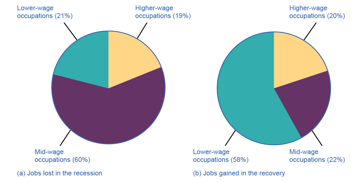
Figure 25.5 Jobs Lost/Gained in the Recession/Recovery Data in the aftermath of the Great Recession suggests that jobs lost were in mid-wage occupations, while jobs gained were in low-wage occupations.
The National Employment Law Project compiled data from the Bureau of Labor Statistics and found that, during the Great Recession, 60% of job losses were in medium-wage occupations. Most of them were replaced during the recovery period with lower-wage jobs in the service, retail, and food industries. Figure 25.5 illustrates this data.
Wages in the service, retail, and food industries are at or near minimum wage and tend to be both downwardly and upwardly “sticky.” Wages are downwardly sticky due to minimum wage laws. They may be upwardly sticky if insufficient competition in low-skilled labor markets enables employers to avoid raising wages that would reduce their profits. At the same time, however, the Consumer Price Index increased 11% between 2007 and 2012, pushing real wages down.
The Two Keynesian Assumptions in the AD/AS Model
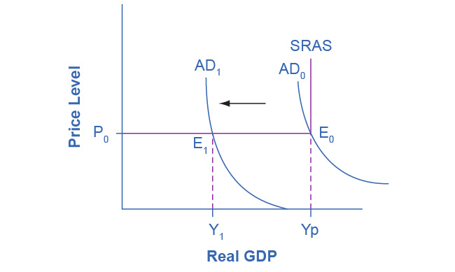
Figure 25.6 is the AD/AS diagram which illustrates these two Keynesian assumptions—the importance of aggregate demand in causing recession and the stickiness of wages and prices. Note that because of the stickiness of wages and prices, the aggregate supply curve is flatter than either supply curve (labor or specific good). In fact, if wages and prices were so sticky that they did not fall at all, the aggregate supply curve would be completely flat below potential GDP, as Figure 25.6 shows. This outcome is an important example of a macroeconomic externality, where what happens at the macro level is different from and inferior to what happens at the micro level. For example, a firm should respond to a decrease in demand for its product by cutting its price to increase sales. However, if all firms experience a decrease in demand for their products, sticky prices in the aggregate prevent aggregate demand from rebounding (which we would show as a movement along the AD curve in response to a lower price level).
The original equilibrium of this economy occurs where the aggregate demand function (AD0) intersects with AS. Since this intersection occurs at potential GDP (Yp), the economy is operating at full employment. When aggregate demand shifts to the left, all the adjustment occurs through decreased real GDP. There is no decrease in the price level. Since the equilibrium occurs at Y1, the economy experiences substantial unemployment.
Figure 25.6 A Keynesian Perspective of Recession This figure illustrates the two key assumptions behind Keynesian economics. A recession begins when aggregate demand declines from AD0 to AD1. The recession persists because of the assumption of fixed wages and prices, which makes the SRAS flat below potential GDP. If that were not the case, the price level would fall also, raising GDP and limiting the recession. Instead the intersection E1 occurs in the flat portion of the SRAS curve where GDP is less than potential.
The Expenditure Multiplier
A key concept in Keynesian economics is the expenditure multiplier. The expenditure multiplier is the idea that not only does spending affect the equilibrium level of GDP, but that spending is powerful. More precisely, it means that a change in spending causes a more than proportionate change in GDP.
The reason for the expenditure multiplier is that one person’s spending becomes another person’s income, which leads to additional spending and additional income so that the cumulative impact on GDP is larger than the initial increase in spending. The appendix on The Expenditure-Output Model provides the details of the multiplier process, but the concept is important enough for us to summarize here. While the multiplier is important for understanding the effectiveness of fiscal policy, it occurs whenever any autonomous increase in spending occurs. Additionally, the multiplier operates in a negative as well as a positive direction. Thus, when investment spending collapsed during the Great Depression, it caused a much larger decrease in real GDP. The size of the multiplier is critical and was a key element in discussions of the effectiveness of the Obama administration’s fiscal stimulus package, officially titled the American Recovery and Reinvestment Act of 2009.
Access for free at https://openstax.org/books/principles-economics-3e


